Machine Learning From Scratch - Part 1, Perceptron

---

This is the first article in a series in which we'll explore AI from the ground up with a series of sports-focused interactive articles. They will use Google Colab to the max extent possible so you'll be able to modify the algorithms and data as you see fit to gain some additional understanding of the topics we cover.

The topics and progression of these lessons are based on the content featured in MIT's undergraduate-level 6.036 Introduction To Machine Learning course. We'll be using new datasets and Colab files, though, to fit our sports theme. Some number of years ago I was on the 6.036 course staff, so I'll draw on that in these articles. For more practice with these concepts, I highly recommend checking out the MIT 6.036 Open Courseware page, where you can see the actual lectures and homework exercises from the class.

Perceptron

The "perceptron" algorithm was one of the first big ideas in artificial intelligence research. It has roots in a 1943 paper by Warren McCulloch and Walter Pitts, but was first truly introduced in a 1958 paper by Frank Rosenblatt. Perceptron is a supervised learning algorithm for binary classification problems. Binary classifiers are functions that place inputs into two classes. This could be a problem like "given a player's career statistics, predict whether they'll make the Hall of Fame or not" or "given a team's field goal and three point shooting percentages, predict whether they won the game or not". These problems come up in a wide variety of places, from medicine to natural language processing. Perceptrons are not the newest or most powerful way to solve these problems, but developing an intuition for how they work can really help when working with larger, more complex models.

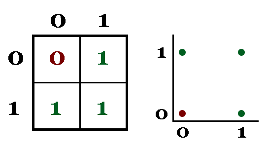
Let's look at a simple case first. The OR function in electrical engineering and computer science has two binary inputs (0 or 1) and one binary output that is 0 when both inputs are 0 and 1 when either output is 1. Graphically, it looks something like this:

We can train a classifier using the perceptron algorithm on this data. We can use the inputs to OR as inputs to perceptron, and the output of the OR function (0 or 1) will be our target class. For consistency, we'll use classes -1 and 1 instead. A quick review of notation: x represents a d x 1 vector of input data, θ (theta) represents a d x 1 vector of weights that we'll learn through this algorithm, θ₀ (theta naught) represents a scalar offset, y represents a scalar label (the true value) and h is the scalar that we predict (-1 or 1). In our notation, superscripts represent elements of a vector, so θ⁰ represents the first element of the θ vector. With that out of the way, let's look at how our perceptron "nodes" will look:

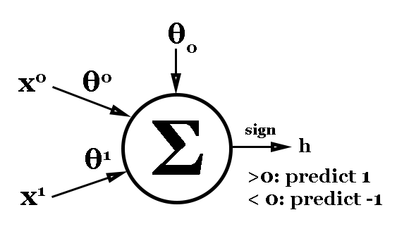
We have the two elements of our input on the left (the two inputs to the OR function) with weights θ⁰ and θ¹ applied to them. θ₀ is our scalar offset that is added to the weighted inputs. That produces our prediction h, which we can compare to the truth label y. To convert the sum value to a class prediction, we'll use the sign function, which outputs -1 if the input is less than 0, 0 if the input is 0, and 1 otherwise.

The Algorithm

Now let's take a look at our algorithm:

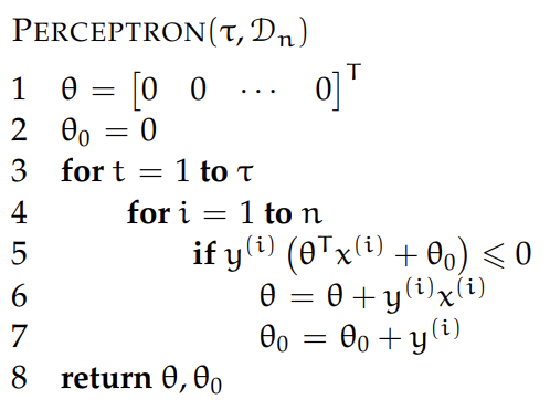
We start by initializing our classifier values to 0. For τ iterations, we loop through every item in the dataset. Look at line 5 carefully - this line says that if and only if our current prediction is incorrect, we'll make an adjustment to our weights. We adjust the weights by "shifting" the classifier in the direction of the true value. Specifically, we adjust θ by a factor of y⁽ⁱ⁾ · x⁽ⁱ⁾ and θ₀ by a factor of y⁽ⁱ⁾.

We continue until we complete all of our iterations or we have a classifier that does not make any errors on the data. That's it! Theoretically our algorithm will always find a classifier that does not make any errors if one exists, although it may take a while. Now let's try it on our problem.

Here, I highly recommend opening the Google Colab notebook associated with this article and running the code yourself. No installation required!

We calculate θ = [[2, 2]] and θ₀ = -1. That classifier is shown by the line below:

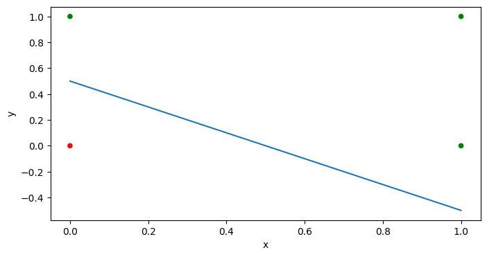
This classifier does in fact achieve 100% accuracy! You can verify for yourself by manually calculating h for each of the points.

Challenge: our code up until this point is based on the OR function, but try adjusting the data to train a classifier on the AND function. For an added challenge, try the exclusive OR (XOR) function (and see more below on how that changed the historical course of AI).

Up until this point, we've seen a basic implementation of the perceptron algorithm and applied it to a simple dataset. Now let's try using it on a more complex (and interesting) problem: predicting the winner of an NBA game based on shooting percentages.

The 2022 NBA Finals

In the 2022 NBA Finals, the Golden State Warriors and the Boston Celtics played to an eventual 4-2 Warriors victory. Leading up to the series, there was a lot of discussion on each team's heavy use of three point attempts in their offense. Conventionally, teams that shoot a lot of three-pointers are perceived as being "streaky", and as a result those teams might not be trusted in the playoffs. Both Golden State and Boston were in the top 10 three point attempts per game in 2022, which makes this Finals matchup a particularly interesting problem.

So did three-point shooting "streakiness" cost Boston a title? Let's use perceptron to train classifiers to predict whether a team won based on their field goal (2 point shots) and 3 point shooting percentages. We'll see how the correlation between 3 point percentage and winning compares to that of field goal percentage.

As a note, this article is more about introducing perceptron and less about a rigiorous statistical analysis of the problem; that will have to wait until we have a more powerful model. We'll see later in the article that perceptron is limited in the types of problems that it can solve.

First, let's load the data. I used an excellent dataset from Kaggle that has game stats for all NBA games from 2004-2022. Then we'll select the 2022 Finals games from the dataset based on the date range.

Now let's sort the data by team and get just the fields we're interested in.

Now let's plot the data. First, Golden State:

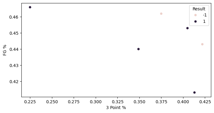
Now Boston:

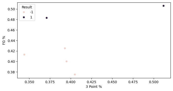
Now that we've plotted the data, let's use perceptron to train a classifier. Let's start with Boston's data:

The data is linearly separable, so perceptron was able to find a solution! Let's plot the classifier.

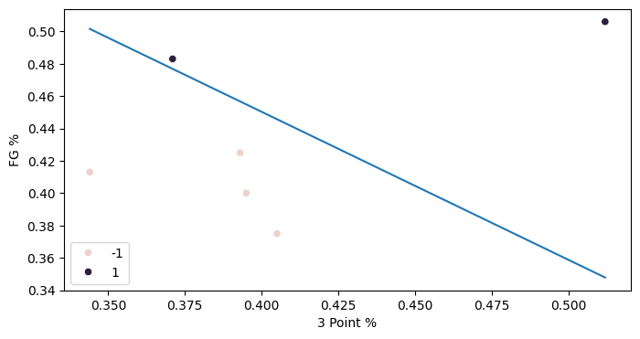
Our classifier achieves 100% accuracy! Looking at the data, though, is it the classifier that you would draw by hand if you were creating a classifier manually? One thing we can see is that there is a small distance between some of the points and the classifier, so a small adjustment would cause it to misclassify that point. That is called the "margin" of the classifier, and in the future we'll see techniques (called "maximum margin classifiers") that allow us to create more robust classifiers.

From this classifier, we can gain some insights into our question on whether three point-reliant teams are "streakier" in the playoffs. This classifier weighs field goal percentage and three point percentage about equally, looking at the components of theta. According to this classifier, then, there is approximately a 1 to 1 tradeoff between field goal and 3 point shooting for a team to be predicted to win. As long as a team shoots well in one area, they will be predicted to win. We can see that the Celtics' four losses in the series came in games where both shooting percentages were low.

Of course, there are many, many limitations to this analysis. We're only looking at one series (6 games total), and we have only trained our classifier on two pieces of data. We are limited to linear classifiers, too. In this next section, we'll try to train a classifier on Golden State's data and encounter an even more fundamental limitation of perceptron.

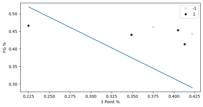
This data isn't linearly separable, and as a result perceptron can't train a classifier that separates this data. The classifier that is does train, though, isn't very satisfying either. It achieves a low accuracy, correctly classifying only 50% of the samples. That's because perceptron doesn't guarantee anything in the case that the data isn't linearly separable. That results in a not-so-great classifier here and actually stunted AI research and development in an "AI winter" after Marvin Minsky published Perceptrons in 1969 and demonstrated that single-layer perceptrons were incapable of solving linearly inseparable problems. Backpropogation had not yet been invented, and so there was just no way to train multi-layer perceptrons.

Conclusion

That concludes our dive into perceptron. It's helpful to understand what this algorithm can do, especially as we dive into more complicated models like Support Vector Machines (SVMs) and neural networks.

With that, feel free to use this code to explore different parts of the NBA dataset! Try different stat fields, playoff series, or anything else you can think of.